Modelling and Model Building

…using the example of our study: “Identification of different factors associated with Covid-19 deaths in Europe during the first pandemic wave”

A large group of statistical techniques designed to explain past data and also to predict future data is statistical modelling. This means that for a given data set with very different variables, one finds a mathematical structure that represents this data set as well as possible, firstly in a purely formal way. This procedure can be used to examine the influence of different variables on an outcome variable. In the language of modelling, the variable that one wants to explain is the dependent variable or criterion or outcome variable, and the different variables that are supposed to contribute to the clarification of this one variable are several independent variables resp. predictors.

I use our recently published modelling study [1] as a concrete example. It was conceived by me, I calculated the first analyses, then my colleague Rainer J. Klement got involved, who as a physicist is much more nimble in dealing with such models than I am.

In this study, we used the deaths of people who died from Covid-19 in the first wave of the 2020 SARS-CoV2 pandemic as the dependent variable (outcome variable or criterion variable). We wanted to know: Which influences on this variable are particularly important, which are rather negligible, and how much of the variation we can explain with the variables we chose as predictors. Technically, this is called the explanation of variance of this outcome variable. Or, to put it another way: which influences contribute to the variation in Covid-19 deaths across European countries?

That the deaths from and with SARS-CoV2 cannot be explained simply by the virus alone is shown by the simple fact that death rates standardized to population vary widely across European countries. If the virus alone were the cause, then death rates standardized to 100,000 people would have to be about the same on a given date. They aren’t. That became clear quite quickly. It also quickly became clear that there must be a variety of other reasons for the different Covid-19 death rates in a country, besides the virus. Because, small example: Belgium, which shares a border with Germany, had by far the highest Covid-19 death rates in the first wave and Germany by far the smallest. If all deaths were exclusively due to the virus and if the SARS-CoV2 epidemic were the only cause of deaths, then the deaths in both countries – always calculated on the same number of people – would have to be the same. Because a virus cannot be stopped by a border, especially since all “measures” came too late anyway.

That is the motivation for this specific modelling study. For all modelling in general, we observe variation, technically speaking variance, in a particular parameter or variable, in this case the number of Covid-19 deaths per country. We want to know how this variation comes about. In other words, we want to know which possible variables are involved in this variation or which variables have an influence on it.

For those who don’t know the basic principle of modelling, preliminarily, a look at my methodology blog on “Modelling” may be of value. With that knowledge, it is easier to understand what we did in this modelling study, in which we tried to understand which variables have an impact on the variation of Covid-19 deaths in the first SARS-CoV2 wave in early 2020.

Modelling variables potentially affecting Covid-19 deaths in Europe

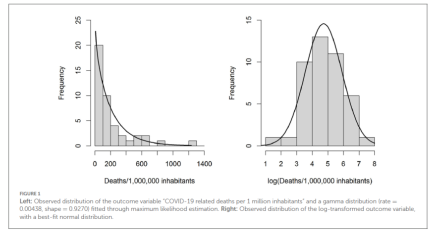
So, our criterion or outcome variable was the rate of Covid-19 deaths in each European country during the first wave of the SARS-CoV2 pandemic. We used data from 43 European countries at the cut-off date of August 20, 2020, which was the day when the first wave was pretty much over everywhere and was chosen somewhat pragmatically. We used the deaths counted up to that date attributed to Covid-19 from the publicly available database as provided by the Our World in Data (OWID) website.

The distribution of these variables is not normally distributed, but follows a gamma distribution fairly closely (see Figure 1, left). If one performs a logarithmic transformation of this variable, then it follows a normal distribution reasonably usefully (Figure 1, right).

We therefore chose a dual analytical approach, the first formulated in the protocol as the main analysis, the second as a sensitivity analysis.

Protocol

By the way, protocols are project descriptions in which the most important evaluation and analysis steps are defined before any evaluations are carried out. I always formulate protocols by default and make them publicly available before a study begins, mostly on the Open Science Foundation platform. For clinical trials, this has been standard practice for some time and there protocols are kept in appropriate trial registries in a database (e.g. clinicaltrials.gov) so that at the end you can be sure that the authors followed the guidelines. In this case, I also created a protocol (https://osf.io/x93np/; there is also an update and an analysis script). In the meantime, some improvements have been made, which we have mentioned in the publication.

Analytical strategy

In this case, the modelling served us to understand whether and which variables have an impact on death rates. Therefore, we formulated different models with different levels of complexity. We computed generalized linear models on a gamma-distributed criterion variable. Such models can be understood like simple linear models, with the difference that the variables are not connected with a simple additive linear link, but are linked as a logarithmic function. Because they are somewhat more complex, their results cannot simply be interpreted directly. It is true that one can also calculate an R²-like characteristic value for them, the so-called Kullback-Leibler R² value, which one can interpret as a percentage of the variance explained. But to make the data easier to interpret, we also ran a linear model on a log-transformed target variable. The results are very similar, showing that the modelling was successful.

The simplest model reproduces the hypothesis: Only the number of cases (standardized to the number of tests, of course) are responsible for deaths. The more cases, the more deaths. Because this variable is very skewed, we have log-transformed. (This is, by the way, a change from my original analysis and description [2]. If you log-transform this variable, then the model becomes better and the variance explained increases. Whereas with the raw values it was only 7% variance explained, with the log-transformed values it is 20% variance explained).

Non-Pharmaceutical-Interventions (NPIs)

Another variable of interest is the impact of the “measures”, technically “non-pharmaceutical interventions” (NPIs), popularly known as “lockdown”. In reality, these “measures” consist of a bundle of possible interventions, from school closures, to border closures, curfews, shop closures, mandatory masking, closing of cultural spaces and restaurants, to strict orders to stay home. The Blavatnik School of Policiy at Oxford University provides a tracker that describes the severity of these measures for all countries of the world in a value standardized to 100% (0: no measures at all; 100: maximum conceivable measures). This value changes and is adapted weekly. In our analysis, this variable emerges as the Government Response Severity Index (GRSI), and as the mean severity in a country over the period of interest.

The second model thus focused on the effectiveness of policy responses.

Flu vaccinations, vitamin D status, hospital beds

The third possible model uses some medical variables in addition to the number of cases, namely the percentage of the elderly population vaccinated against influenza. This was motivated by an interesting study that found a positive association between influenza vaccination and Covid-19 death rates [3]. We included in this model as a possible protective factor, corroborated by various studies, the vitamin D supply of the population, which we had compiled from different studies, as well as the number of hospital beds per 100,000 population.

Population parameters

Because Covid-19 primarily affects older people, we formulated a model using life expectancy in a country and the number of older people in the population as predictors, in addition to the number of cases and vitamin D status.

Risk factors

Risk factors, such as coronary heart disease and diabetes, as well as smoking as a possible risk or even protective factor [4, 5] went into another model, in addition to case number and vitamin D status.

Country-specific factors

Finally, we built a model in which country-specific factors such as population size and density, percent of the elderly, gross domestic product, and development index entered in addition to the log-transformed standardized cases and vitamin D status.

Full model and data-driven model via LASSO analysis

Finally, we still analysed the full model with all 13 variables and computed a data-driven model using a relatively novel analysis method, abbreviated as LASSO [6]. LASSO stands for “Least absolute shrinkage and selection operator”, or: an operator that sets the least significant predictors to zero and selects those that then gain significance.

The full model is simple to understand: It simply uses all variables. The LASSO model is data-driven. Here, in an iterative process, all variables are set to zero except one. Of these, the one that makes the most important contribution to variance explanation is chosen first. Then this iterative process is repeated for the next remaining variables, and so on. This is initially a purely exploratory procedure, but it has the advantage that it does not require multiple modelling. In this way, one can identify which variables are really important and then formulate a model for these variables thus selected.

Selecting models and the Akaike Information Criterion

These 8 models produce differently good fits. So how does one decide? The so-called Akaike Information Criterion (AIC), proposed by the Japanese statistician Akaike, helps here. It is an absolute number that is not very meaningful on its own. It takes into account the goodness-of-fit of a model and the number of parameters required for it. A model with a larger number of parameters is “penalized” in that the AIC increases. Therefore, one can use the AIC to determine the relative model goodness.

Of a class of models, the best is the one that has the comparatively lowest AIC.

We have presented the analysis results and the corresponding model parameters in Tables 1 and 2 of the original publication.

I reproduce here in Table 1 only the most important results.

Modell No und Variablen im ModellModel No and variables in model	Regression weight b	Significance of b p-. Value	KL-R2	AIC	Delta AIC
Model 1			0.2	541.3	36.2
Cases	0.6	.0008
Model 2			0.26	538.5	33.4
Cases	0.6	.0005
GRSI	0.04	.035
Model 3			0.47	524.8	19.7
Cases	0.73	2*10-5
Vitamin D	-0.3	.4
Beds	0.025	.7
Flu vaccinations	0.032	3*10-5
Model 4			0.45	527.5	22.43
Cases	0.73	3*10-6
Vitamin D	-0.47	.11
Life expectancy	0.19	4 * 10-5
Proportion elderly	-0.033	.5
Model 5			0.49	524.9	19.8
Cases	0.71	8*10-5
Vitamin D	-0.36	.2
Smokers (%)	-0.007	.8
CVD deaths	-0.999	.02
Diabetes prevalence	-0.09	.18
Model 6			0.48	527.5	22.42
Cases	0.96	6*10-6
Population density	0.22	.058
Life expectancy	-0.011	.88
GDP	2.6*10-5	.09
HDI	1.94	.7
% elderly	0.08	.2
Model 7			0.67	524.2	19.1
Cases	0.97	2*10-6
GRSI	0.03	.055
Vitamin D	-0.716	.043
Flu vaccination	0.02	.0055
Life expectancy	-0.05	.7
Population density	0.09	.4
% smokers	-0.014	.5
CVD mortality	-0.04	.9
Diabetes prevalence	-0.06	.4
Beds	0.03	.6
GDP	4*10-8	.005
HDI	-2.5	.6
% elderly	0.09	.14
Model 8			0.68	505.1	–
Cases	0.84	9*10-7
GRSI	0.02	.07
Vitamin D	-0.7	.02
Flu vaccinations	0.02	.0002
Population density	0.13	.2
GDP	3*10-5	.007

As I said, the linear regression on the log-transformed criterion variable yielded almost the same results, so I won’t go into that. Those who are interested can have a look at the original table. Also, it should be mentioned: we replaced missing cases with an interpolation algorithm because we did not have data for all variables for each country and because missing values exclude a case from the analysis, which reduces statistical power. To check whether this procedure had an impact, we adjusted the analysis for the data for which all cases were available and got pretty much the same results; again, I do not present this separately here. The table is in the original publication.

Let us now turn to the models and what they tell us. Let’s start with the worst and simplest, Model 1, which uses only the standardized number of cases as a predictor. This model tests the hypothesis of whether the number of cases is sufficient as a predictor. Obviously, this is not the case. Both model fit, captured by the Akaike information criterion, and variance resolution are worst for this model. The difference in AIC from the best model is the largest, 36.2. It is usually assumed that AIC differences below 5 signal roughly equivalent models, and above 15 rule out a model as implausible.

The best model is clearly the data-driven model number 8 found by the LASSO regression. It is able to explain more variance with only 6 variables, namely 68%, than the model that uses all variables, namely model 7. This also has a much worse value, with an AIC difference of 19.1 points. The same applies to all other models, which I therefore do not even discuss.

The number of cases also enters as a significant and strongest predictor in the best model number 8. The second-strongest predictor is the supply of vitamin D in the population. This predictor is negative, i.e. protective and significant. The data on vitamin D supply are intrinsically poor because there are few good population-based studies for all European countries. Therefore, we dichotomized the variable into sufficient or non-sufficient. Of course, this is extremely coarse-grained. We were all the more surprised that we still found a relatively strong effect. We followed up the analysis with latitude and saw that this alone did not explain the effect. The predictor that comes third, measured by the size of the regression weight, is population density: the larger, the more cases. However, this predictor is not significant, so it plays a minor role despite its size.

The rate of influenza vaccination coverage among the elderly population is a highly significant predictor, although the effect is rather small: the more influenza vaccinated elderly in a country, the more Covid-19 deaths.

How can this be understood? For one thing, it is conceivable that there are still background variables that we have not captured that are driving this impact. In any case, the ones we have captured do not play a role in it. This is because the variable is a significant predictor even in the full model, in which all variables enter, and in all other models in which we have introduced it. It is univariately related only to life expectancy (r = .56) and negatively related to cardiovascular mortality (r = -.57), so the more flu vaccinations, the less cardiovascular mortality in a country. But: the more flu vaccinations, the more Covid-19 mortality. We seem to have a choice between plague and cholera, so to speak. We don’t seem to be able to protect ourselves against everything at once. On the one hand, there is the phenomenon that pathogens seem to form a kind of symbiotic ecosystem. If you expel one, others will come. On the other hand, it could be that the vaccination against influenza keeps the immune system busy for a while [7]. During this time, another pathogen might more easily overcome the immune system. A very good randomized study in children showed: children vaccinated against influenza had significantly less risk of getting influenza, but a fourfold increased risk of getting other respiratory infections. [8]

Gross domestic product is a typical example of a highly significant but factually unimportant predictor in this model, because its numerical value is extremely small, 0.00003: the more a country generates, the greater the Covid-19 mortality in that country.

Most interesting to me from a conceptual point of view is the fact that the Government Response Index GRSI, which maps the harshness of the measures, is a weak but positive predictor. That is, the stronger the measures, the more deaths. If the measures had done anything positive in the first wave, we would have expected a negative sign here. This is not the case. The predictor is not particularly significant either, so it does not play a major role, but if it does, it is an inglorious one. We had already shown in another publication that the ill-fated modelling study that supposedly proved that Germany’s lockdown was necessary [9] used an incorrect data basis [10]. In my view, the data basis for the effectiveness of lockdowns and measures is poor. This new analysis corroborates that finding.

Summary of our Covid-19 mortality modelling

So we now know: in the first phase of SARS-CoV2 spread, case numbers, standardized to the number of tests, were an important predictor, explaining about 20% of the variance. However, the best model with 6 variables can explain a total of 68% of the variance. The harshness of the measures matters: the harsher the measures, the more deaths; the closer together the population lives, the more deaths; the better the supply of vitamin D, the fewer deaths; the higher the flu vaccination coverage among the elderly, the more deaths; the higher the GDP, the more deaths. This leaves 32% of the variance unexplained. We know that the famous comorbidity variables (prevalence of diabetes, of cardiovascular disease and of smoking) do not play a big role in this; because models in which we have introduced them are less good at explaining the variance. But of course, it could be that we have missed other important variables: how happy a country is on average, what the level of anxiety is, or the rate of depression. We have not checked these. Others are welcome to do so. Our data set is available. But I think: 68 % variance clarification is already pretty good. And if one were to take this information seriously and, for example, conduct a nationwide campaign to ensure that the population has an adequate supply of vitamin D, or if one were to make appropriate material available to every household, then that would be guaranteed to be more effective than mandatory masks in trains and schools. That much can be said. For compulsory masks are part of the GRSI, and it plays rather an inglorious role.

Sources and literature

1. Klement RJ, Walach H. Identifying factors associated with Covid-19 related deaths during the first wave of the pandemic in Europe. Frontiers in Public Health. 2022;6th July 2022. doi: https://doi.org/10.3389/fpubh.2022.922230.
2. Klement RJ, Walach H. Low Vitamin D Status and Influenza Vaccination Rates are Positive Predictors of Early Covid-19 Related Deaths in Europe – A Modeling Approach. Zenodo. 2021. doi: https://doi.org/10.5281/zenodo.4680691.
3. EBMPHET  Consortium. COVID-19 Severity in Europe and the USA: Could the Seasonal Influenza Vaccination Play a Role? SSRN. (7/6/2020). doi: https://doi.org/10.2139/ssrn.3621446
4. Patanavanich R, Glantz SA. Smoking is Associated with COVID-19 Progression: A Meta-Analysis. medRxiv. 2020:2020.04.13.20063669. doi: https://doi.org/10.1101/2020.04.13.20063669.
5. Farsalinos K, Eliopoulos E, Leonidas DD, Papadopoulos GE, Tzartos S, Poulas K. Nicotinic Cholinergic System and COVID-19: In Silico Identification of an Interaction between SARS-CoV-2 and Nicotinic Receptors with Potential Therapeutic Targeting Implications. International Journal of Molecular Sciences. 2020;21(16):5807. PubMed PMID: doi: https://doi.org/10.3390/ijms21165807.
6. Tibshirani R. Regression Shrinkage and Selection via the Lasso. Journal of the Royal Statistical Society B. 1996;58:267-88.
7. Cowling BJ, Nishiura H. Virus Interference and Estimates of Influenza Vaccine Effectiveness from Test-Negative Studies. Epidemiology. 2012;23(6):930-1. doi: https://doi.org/10.1097/EDE.0b013e31826b300e. PubMed PMID: 00001648-201211000-00030.
8. Cowling BJ, Fang VJ, Nishiura H, Chan K-H, Ng S, Ip DKM, et al. Increased risk of noninfluenza respiratory virus infections associated with receipt of inactivated influenza vaccine. Clin Infect Dis. 2012;54(12):1778-83. Epub 03/15. doi: https://doi.org/10.1093/cid/cis307. PubMed PMID: 22423139.
9. Dehning J, Zierenberg J, Spitzner FP, Wibral M, Neto JP, Wilczek M, et al. Inferring change points in the spread of COVID-19 reveals the effectiveness of interventions. Science. 2020;369(6500):eabb9789. doi: https://doi.org/10.1126/science.abb9789.
10. Kuhbandner C, Homburg S, Walach H, Hockertz S. Was Germany’s Lockdown in Spring 2020 Necessary? How bad data quality can turn a simulation into a dissimulation that shapes the future. Futures. 2022;135:102879. doi: https://doi.org/10.1016/j.futures.2021.102879.