Our Modelling Study “Influence of Fish Consumption on Students’ PISA Scores” as An Introductory Example
I will soon present our modelling study that attempts to present the variation in Covid-19 mortality rates in the first wave up to summer 2020. To illustrate this method, I use here a study we conducted some time ago [1]. My colleague Volker Schmiedel, who is very interested in the importance of omega-3 fatty acids, gave the impetus for this study. We asked the simple question:
Does the availability of omega-3 fatty acids in a country affect children’s PISA scores?
PISA (Programme for International Student Assessment) is, as is well known, an internationally conducted, standardized test to examine children’s abilities at school. Volker Schmiedel came up with the idea of correlating the fish consumption of a country with the PISA scores of that country and discovered a significant correlation. The simple correlation between fish consumption and a country’s PISA score is r = .57, which is not only significant, but also quite highly so. In fact, surprisingly high. After all, why should fish consumption be related to students’ knowledge at school? The correlation might be understandable only because of the omega-3 fatty acids, which are mainly found in oily fish, but also in dark green plants, algae and everything that feeds on them. It is not easy to measure omega-3 levels in a population. You would have to take blood from a representative sample of the population and determine the omega-3 content in, for example, the membranes of red blood cells. To my knowledge, no one has ever done this systematically across a variety of countries. Fish consumption is easier to measure, it is a so-called proxy variable. Because fish is a main supplier of omega-3 fatty acids. And omega-3 fatty acids are important for us as essential fatty acids. We have to take them in through food because we cannot produce them ourselves. Since the industrial revolution at the end of the 18th century, omega-3 intake has decreased [2]. Omega-3 is not only central to the immune system because it is the precursor substance for all cytokines with anti-inflammatory effects. It is especially important for nerve growth in children and learning in old age. It is also important for maintaining cognitive performance. For example, the level of omega-3 in mothers’ milk can predict the intelligence of schoolchildren to an astonishing degree [3, 4].
For all these reasons, Schmiedel’s consideration was of course very clever: it is possible that the PISA score, as an expression of the cognitive performance level of children, is related, among other things, to how much omega-3 fatty acids they consume, roughly measured by the fish consumption of a nation. Now, of course, the question immediately arises: What influences the PISA score in particular? And if we know that, does fish consumption play a role in addition to that?
The general principle: linear combination of weighted influence of variables
The general mathematical estimation formula for such a question is:
y = a + β1x1 + β2x2 + β3x3 +… βnxn +e. (Equation 1)
“y” here is, in general terms, the variable you want to clarify, i.e., for example, the variation in students’ PISA scores, or in Covid-19 deaths in Europe.
“a” is a constant, or the so-called intercept. Graphically, it would be the point at which a regression line intersects the x-axis, indicating the empirical zero point. One needs this value if one wants to make concrete calculations for single individuals, or if one wants to use a found regression equation in the future or with another data set to calculate values. At the moment, this value is not so important for understanding the general principle of clarifying variation.
The so-called “β” weights are the regression weights or regression coefficients. If they are standardized, i.e. they can assume a distribution between -1 and +1, they are usually rendered with the Greek β symbol. If they are unstandardized, then b is usually noted. They indicate how great the influence of a variable x on the criterion y is. If, for example, a regression weight were only 0.0001, then the influence of the variable with this weight would be understandably very small. If β is very large, e.g. 0.8, then the influence of this variable is also relatively large. If the weight is positive, then the variable has a positive influence: i.e. the greater x, the greater y. If the weight is negative, then the variable has a negative influence: thus, the greater x, the smaller y.
Now you can see immediately from equation (1) that this is a linear combination of variables x1 to xn, basically any number of variables or predictors that can be used to explain y, the criterion. That is the charm of modelling: You can use as many variables as you can collect for the explanation. There is a practical limit: Since these regression weights are not simply found in the open, but have to be estimated by a computationally intensive iteration procedure, you need a correspondingly large number of data sets to be able to make this estimate in a stable manner.
Technically speaking, the least squares method is usually used for this: The computer averages the individual variables, then uses different regression weights while holding everything else constant, squares the difference between the mean and the weighted mean, and does this iteratively until the difference is a minimum. When such procedures still had to be calculated by hand, it was very time-consuming and limited the number of variables for that reason alone. Today, computers can do it in fractions of a second. But you still have to be aware of the fact that the computer only calculates with what is available. And to be able to perform a stable estimation, the computer needs – rule of thumb – about 10 cases per influence variable to be estimated or the associated regression weight β [5].
Then, at the very end of equation (1), we see the “e”, sometimes represented as the Greek epsilon – e -. This is universal statistical language for “error term” or “residual”. This is the portion of the variation that cannot be explained by these variables.
This general principle of linear combination of weighted influence variables to “predict”, i.e. explain, an individual value applies to all modelling. In some regression methods, the combination of the individual prediction terms is more complicated. In non-linear regressions, for example, there are quadratic, cubic or other function terms. In logistic regressions, these regression elements are exponents of Euler’s number e. But the principle is always the same: A set of variables is used to “predict” in an optimal combination a variable to be explained, the criterion or dependent variable, that is, to elucidate as much as possible in its range of variation or variance.
Concretely, using the PISA study:
We collected PISA scores from 64 countries, from which we also had information on fish consumption. In addition, we used data on economic development, in this case gross domestic product (because this indirectly determines how much funding a country has), data on the availability of the internet in a country, as an indicator of technological development, and the breastfeeding rate. All these data are available from public sources and are intuitively and theoretically plausible influencing factors whose impact on a country’s PISA score can be estimated.
It can be seen at this point that the variables one feeds into such a model also depend on the question. This in turn depends on theoretical knowledge and conceptual assumptions, and not infrequently, as in our case, also on the availability of data.
By the way, the individual units, i.e. cases, in this study are not individual children but countries with their PISA averages. Usually in such studies, individuals are the unit of analysis. In the PISA study and also in our Covid-19 modelling, countries are the units of analysis or “cases”.
We have now calculated a linear regression model as described above. I reproduce the original Table III of the publication here as Table 1 and will then explain it:
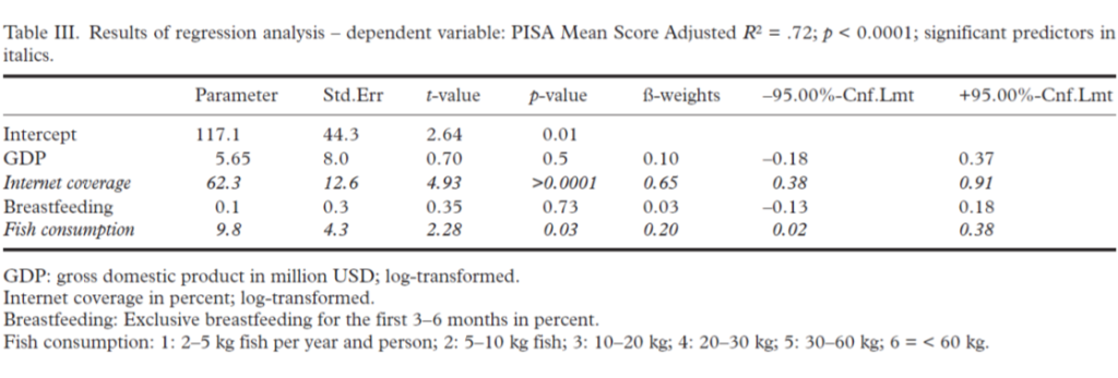
You can see: we used five variables for prediction, GDP-Gross Domestic Product, a country’s internet coverage, the percentage of children in a country who were breastfed, and at the end, a country’s fish consumption, roughly measured in 6 reasonably continuously increasing categories (2-5 kg per person per year, 5-10 kg, 10-20 kg, 20-30 kg, 30-60 kg, and more than 60 kg).
The latter is important because linear regression models have several assumptions. One is that the criterion variables and all other variables must be reasonably normally distributed, and that the variables one uses for prediction must be continuous variables. If they are not continuous but categorical, then you have to recode them into so-called dummy variables, i.e. 1-0 codings (or -1 and +1) for individual categories, which are then continuous again. In our case, I used the fish consumption variable both as a continuous variable and as a dummy-coded variable for the individual categories. The difference is negligible. Therefore, I report the model for the continuous variable in the publication and discuss the potential problem in the discussion because a reviewer had insisted on it.
We see: The model is highly significant and can even resolve 72% of the variance with R2 = .72. This model statistic is the first important finding. It tells us whether the statistical model is firstly significant and secondly how high the multiple correlation R, i.e. the correlation of all variables together with the criterion, is. Squared, each correlation coefficient gives the variance explained. Example: let a person’s intelligence be correlated with his subsequent income about r = .3 – which, incidentally, roughly corresponds to the empirical ratios; then the variance thus elucidated would be r2 = .32 = .09 or 9%.
In our case, R2 = .72 (the multiple correlation coefficient, which describes the influence of several variables simultaneously, is always capitalized). The variance elucidation with 72% is considerable. This is because only 2 variables are needed: internet coverage, which is a proxy for the economic-technical development of a country, and fish consumption. This more detailed insight is the second important insight that statistical modelling provides. It tells us which variables we use in our modelling contribute to this variance explanation, and how much.
You can see from Table 1 above that the beta weight for internet coverage is quite high at 0.65. This variable is also highly significant, while gross national product remains irrelevant as a predictor. This is because internet coverage and gross national product are very highly correlated with each other with r = .87 (this is explained in Table 2 of the publication) and in this case the model uses the variable that is a better predictor. This automatically drops the other out of the equation. I have also done analyses with gross national product only. But these have slightly lower variance explanations.
Now the analytical idea of this analysis would be: if a country’s PISA score can be explained by these social variables (GDP, internet coverage, breastfeeding rate), then fish consumption should be irrelevant as a predictor. What we see, however, is: the breastfeeding rate hardly plays a role. The beta weight of 0.03 is very small and not significant. But fish consumption is a significant predictor at beta = .20.
In fact, one can take a quasi-experimental approach in such analyses and ask, for example: If you control for all social variables, is fish consumption still a significant predictor? In such a case, one proceeds step by step or forces the system to include the social variables first and then, in the last place, or even in the last step, the variable of interest. This is fish consumption here. That’s what I did here, and you can see: Even if you include all the other variables first, fish consumption is still a significant predictor. It explains an additional 4% of the variance. So a model without the predictor “fish consumption” would only have an R2 = .68.
Still high, but lower. This allows us to conclude: When social-economic progress is taken into account, fish consumption, and thus presumably omega-3 availability, is an additional, important predictor. The fact that these variables together can explain 72% of the variance is, in my view, astonishing. Of course, other factors also play a role: how good the school system is, how good the teacher training is, how motivated the teachers are, how large the classes are, how long children sleep, etc. But all of this we did not capture, or rather, we had no data on it. We had data on school satisfaction from some countries and repeated the analysis with school satisfaction for these countries. But the picture did not change, and school satisfaction was not a significant predictor.
I have given the parameters or raw regression weights in the first place in Table 1 above. These are not standardized and provide information on how much a variable would be weighted in an actual prediction calculation.
Then follows the standard error of this estimate. This is needed for the significance calculation, which is kindly supplied by the statistics program. The distribution of these parameters follows the T-distribution, a statistical distribution that is similar to the normal distribution, only steeper depending on the number of observations. From it, we can obtain the probability of error: p. It tells us whether a regression weight has a significant, i.e. has an influence beyond statistical randomness. It is quite possible that a relatively large regression weight is not significant and, conversely, a very small one is significant. This then means: The influence is present, but statistically difficult to distinguish from a random variation. Or: The influence is very small, but clearly beyond random fluctuation.
The standardised beta weights that then follow in the next column can be interpreted as partial correlation coefficients. They represent the correlation of the corresponding variable with the criterion, i.e. in this case with the PISA score of a country, if the influence of all other variables is kept statistically constant or factored out. (For the variables also have correlations with each other, which are then controlled for.)
You can also illustrate the principle graphically in a so-called Venn diagram, which I reproduce here in Fig. 1.
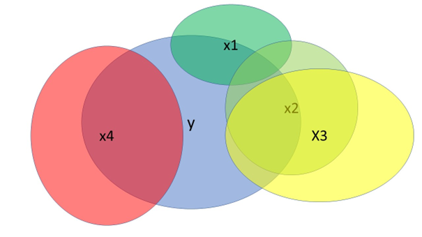
The blue circle y represents our target variable, the criterion. The variables x1 to x4 are possible predictors. They have a certain correlation with the criterion – the overlap range – and often also a correlation with other variables. For example, the own contribution of x2 that area not covered by either x1 or x3 would be relatively small. The own contribution of x3 is also not as high as it first appears, because the correlation with x2 is very high. This is called “collinearity”, a common high correlation. Intelligent modelling checks this and uses, out of 2 possible variables, the one with the highest own explanatory value. In our analysis, this was internet coverage. Variable x4, on the other hand, would have a relatively high explanatory value in this graphical example and its own independent correlation with criterion y, without being related to the other variables. The pure blue of y not covered by other overlapping circles, that would be the proportion of unexplained variance or in the individual case, the residuals.
To understand residuals, it is useful to work through a concrete regression equation. We do this for the examples of China and Qatar from our dataset:
China, the upward outlier in Figure 3 below, has the highest PISA score in our dataset at 567.66 and Qatar the lowest at 308. Breastfeeding rates are similar, as is internet coverage, 87% in Qatar, 74% in China, but GDP is very different, at $100,260 Million for Qatar and $6,747 Million for China (data from 2013). Now you can see in Table 2: I log-transformed the value for the gross national product and for the internet coverage because the data were too skewed and thus achieved an approximate normal distribution. Fish consumption is a 6-level, approximately continuous variable.
| Country | PISA value | Fish consumption | Breastfeeding rate | GDP transf. | Intern. transf. |
| China | 567.66 | 5 | 28% | 8.816 | 4.304 |
| Qatar | 398 | 4 | 29% | 11.515 | 4.466 |
We now use equation (1) and the data from Table 1, which give the original regression weights:
yChina = 117.1 + 5.65*8.816 + 62.3*4.304 + 0.1*28 + 9.8*5 +e =
117.1 + 49.81 + 268.14 + 2.8 + 49 + e =
486.85 +e
yChina– 486.85 = e
567.66 – 486.85 = e
e = 80.81
So the regression equation for China gives a PISA score 80.81 points lower than it actually is. This is the upward outlier in Fig. 3 below, which is pretty much at 80 points, or in the histogram in Fig. 2, the value at the far right of the distribution.
Whoever wishes can now do the same with the data for Qatar and will find that the equation gives a negative error or residual of about -100 points, i.e. Qatar’s PISA scores are estimated by the equation to be about 100 points higher than they are in reality. (“Reality” here means empirical reality.)
It would now be a question of more sophisticated analysis as to why this is the case with these outliers. It could be, for instance, that Chinese data is unreliable. That the school system is much better, etc.
Anyway, this is how you see: Regression equations can be used for individual prediction, for example of new data sets, which is often used in industry in process control. And in this way one also understands the function and arithmetic magnitude of error terms or residuals e. They represent the error in the individual case, and the unexplained variance in the case of a total data set.
Consider prerequisites
Now, one thing to bear in mind about such an analysis is that it will only yield valid analysis results if the preconditions are met. I already mentioned two that one has to check before the analysis: Are the variables reasonably normally distributed? They were in our case. I say “reasonably” because the routines react relatively robustly to a violation of this assumption. If the normal distribution, especially of the criterion variable, is strongly violated, one can use a trick and transform it logarithmically. Then it will often be normally distributed. You can do the same with the other variables.
Furthermore, one takes a look at the residuals, i.e. the unexplained portions, those 28% of the variance, in our case, that cannot be explained by these variables. They must be reasonably normally distributed. Publications often show this graphically in the appendices. Similarly, a plot of the residuals against the predicted values should not reveal any pattern. For if patterns are discernible, the assumption that the relationship is nonlinear is likely.
I reproduce here in Figures 2 and 3 the histogram of the residuals and the plot of the residuals vs. the predicted values:
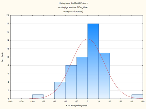
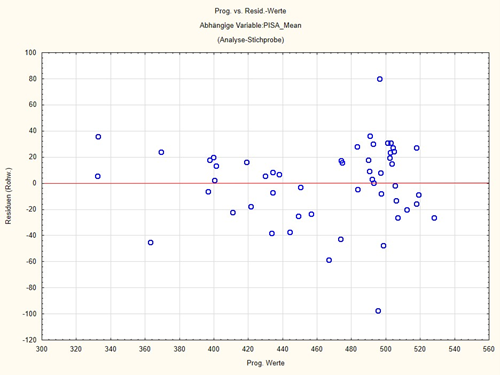
You can see from Fig. 2: the residuals are reasonably normally distributed around 0. There are some outliers where the predicted PISA score is almost 100 points too high or too low. But otherwise the model fits quite well. You can also see these outliers in Figure 3. You can also look at the outliers with statistics programs, in our case the downward outlier is Qatar and the upward outlier is China. But otherwise, no pattern is discernible in this plot. A pattern would be something like a cloud rising continuously to one side.
The analytical concepts of linear models
Linear models can thus serve several purposes:
- They are used to estimate the significance of possible predictor variables or independent variables and thus their influence on the criterion or independent variable. In clinical studies and experiments, for example, this can also be used to detect the influence of an experimental manipulation. This is then represented by a categorical dummy variable that is 1/0-coded. The influence of a variable is shown by the size (and of course the significance) of the regression weights. With standardized regression weights, denoted by b, this can be done immediately. This is because the regression weights can be interpreted as partial correlation coefficients, i.e. as the correlation of the predictor variable with the criterion variable when the influences of all other variables are statistically controlled. In our example: fish consumption in a country correlates with the country’s PISA score (and vice versa) with 0.20 if all the other variables in the equation are statistically controlled. That is, when their influence on fish consumption has been removed. Thus, one can use the magnitude of β as an estimator for the influence of a variable. In the picture of Fig. 1: It is the overlaps of a circle with the y-circle without the share of other overlapping circles. If, as is often the case with other regression models, the weights are not standardized, then one can use the relative size as a guide, i.e. the size relative to all other regression weights.
- One can use a regression equation to make predictions for individual cases. This is mainly used in process control, when you have determined a regression equation from standardized data sets that you can then apply to new data sets. For analytical research, this is rather less important. I used this approach above to make clear what role residuals play.
- If you solve the entire equation over all data sets and estimate the statistical model as a whole, then you can see how well the model fits the data overall. We saw from the model of the elucidation of the PISA score that a relatively high explanation of variation is possible with this model. This analytical step is called “goodness of fit”, or “model goodness”, or predictive power of the model. It has two main components: an R2 value and F or Chi2 value with an associated p-value or probability of error. The R2 value is the squared multiple correlation coefficient, i.e. the correlation of all variables used in the equation together with the criterion or dependent variable. It is squared because a squared correlation coefficient can be interpreted as the proportion of variance explained or variation explained. The multiple correlation coefficient R2 thus explains how much variance or variation, e.g. in the PISA scores of individual countries, we can explain with the given variables, in our example 72% of the variation in the PISA scores. The fact that we do not know and have not recorded all the variables that have a possible influence is expressed in the unexplained variance and, at the individual level, in the error terms or residuals e.
This R2 value is distributed according to the F or the chi-square distribution, depending on the model. These distributions are known. Therefore, one also normalizes them. Then one can define the area under the curve as “1” and thus as probability. Then one can also define the area from a certain ordinate as a probability, and if a certain value exceeds a limit or the area to the right of it is very small, then the probability of such a value is very small. This can then be used to determine the probability of error of an empirically found R2-value.
The overall model thus has two important ratios: the R2-value, the size of the variance explanation, and the significance or statistical probability of error of this value.
In fact, it depends on the size of the correlation, but also on the size of the data set, whether a multiple correlation coefficient R2 is significant. I have already dealt with this several times under the topic of “power” or “statistical power”. This also applies here: With a very large number of cases or data sets, one can also get very small and irrelevant correlations, e.g. R2 = 0.002, i.e. 0.2 % of the variance explanation, significant. Conversely, a large correlation may miss significance if the data set is small. Ideally, we expect high variance elucidation to be significant at the same time.
In research, we are mostly interested in 1. – size of associations of predictors with the dependent variable or outcome – and 3. – amount of variance explained by a model.
In medical and social science research, it is rare to find models that explain more than one-third to one-half of the variance, and usually require something between 3 and 10 variables at least – and a factor of 10 to 20 more cases.
Large epidemiological surveys usually have many thousands of cases and can therefore also model numerous possible influencing variables or predictors. The problem with all these studies is always: you never know whether you have captured the really interesting and important variables and whether you are not missing an important influencing variable. There is only one indirect way to estimate this, namely R2, the amount of variance explained. If this is high, the probability that one has overlooked something important is low.
In our example above, we had 5 variables and 64 cases, so enough power to estimate the parameters.
We have now discussed classical linear regression using this example. This is the basic structure. It can be extended in very different ways, and the principle is always basically the same.
When one evaluates clinical trials or experiments, one usually introduces the variable that codes for the intervention as an additional predictor alongside predictors of interest. If this is significant, then you know that the intervention had an impact, and you can also estimate the strength of the impact.
If the distribution of the criterion or target variable does not follow the normal distribution, then the regression models are formalized slightly differently. One then speaks of the “generalized linear or non-linear model”. For example, one can calculate regressions on variables that follow a Poisson distribution, a gamma distribution, a logistic or other distribution. Then the predictors are not coupled with a simple linear combination, but are either first transformed with a logarithmic transformation and then additively combined. In the case of regressions that follow a logistic distribution, the regression elements are linearly connected exponents of the natural number e. In the case of nonlinear regressions, the regression elements are fitted to a suitable power.
But the important thing is to understand the principle I was trying to convey here: it is always a linear, or non-linear, combination of weighted predictive terms to resolve variance in a criterion. Sometime in the 1960s, it was also shown arithmetically that the analysis of variance and the regression analysis, which had been so popular until then, are conceptually equivalent [6]. Since then, one speaks of the “General Linear Model” or the “Generalized Linear Model”. It is perhaps the most powerful tool for elucidating multiple influences on a variable of interest.
Sources and literature
- Schmiedel V, Vogt H, Walach H. Are pupil’s “Programme for International Student Assessment (PISA)” scores associated with a nation’s fish consumption? Scandinavian Journal of Public Health. 2017;46:675-9. doi: https://doi.org/10.1177/1403494817717834.
- Moffett JR, Ives JA, Namboodiri AM. Fatty acids and lipids in neurobiology: A brief overview. In: Watson RR, editor. Fatty Acids in Health Promotion and Disease Causation Urbana, IL: AOCS Press; 2009. p. 517-43.
- Weiser M, Butt CM, Mohajeri MH. Docosahexaenoic acid and cognition throughout the lifespan. Nutrients. 2016;8(99). doi: https://doi.org/10.3390/nu8020099.
- Hibbeln JR, Davis JM, Steer C, Emmett P, Rogers I, Williams C, et al. Maternal seafood consumption in pregnancy and neurodevelopmental outcomes in childhood (ALSPAC study): an observational cohort study. The Lancet. 2007;369(9561):578-85. doi: https://doi.org/10.1016/S0140-6736(07)60277-3.
- Barth M. Konzeption und Evaluation multipler Regressionsanalysen in der anwendungsorientierten klinisch-psychologischen Forschung. In: Strauss B, Bengel J, editors. Forschungsmethoden in der Medizinischen Psychologie. Jahrbuch der Medizinischen Psychologie 14. Göttingen: Hogrefe; 1997. p. 146-60.
- Wittmann W. Evaluationsforschung. Aufgaben, Probleme und Anwendungen. Berlin: Springer; 1985 1985.