(25) Models And Causality

Can we say anything about causality with such models? For example, can we say that flu vaccinations causally increase Covid-19 death rates, or higher vitamin D levels causally decrease Covid-19 death rates? In a technical methodological sense, you can’t. Because we only have cross-sectional data in front of us. It would only work if we had a strong theoretical model at the same time. We can rule out reverse causality: Covid-19 death rates do not drive up vaccination rates among the elderly (because flu vaccination data are mostly pre-pandemic), and we can also rule out that Covid-19 death rates lower vitamin levels. Because there is no plausible theory for that. It is conceivable, however, that Covid-19 death rates drive the GRSI: The more deaths in a country, the stronger the government’s response. However, they are usually mistaken in thinking that the measures have something to do with the dynamics of deaths. Rather the other way round: the dynamics of the measures are driven by the dynamics of the death rates.

This leads me to a few thoughts on causality and how, at best, it can be clarified in the context of modelling. First, a few general remarks on causality.

Causality

In my opinion, the still cleverest and as yet unsurpassed analysis of causality is by David Hume [1], who, incidentally, most probably got it from William Ockham [2, 3, p. 629] and if he didn’t crib it there, he was simply a very clever man who got about the same result independently.

Ockham, in his Commentary on Aristotelian Physics, which he must have written while teaching at Oxford in the early 14th century, defined cause as follows: “We must assume a proposition which seems evident, and that is this: ‘This is the cause of another thing: if it is not present – all else unchanged – neither is the thing; if it is present, then the thing is also given.‘” [3, p. 629] This is a purely correlative, negative formulation: if the cause is not present, neither is the thing in question. If the cause is present, the fact is also present. Example: Light is the cause of seeing. If there is no light, we do not see. If it is there, we see. Or: Where there is no smoke, there is no fire. If there is fire, there is smoke.

Ockham, in the course of his criticism of the scholastic concepts, got rid of all essences, entities and forces that would mediate causes, for instance, and formulated the concept of cause in purely correlative terms.

Hume took up this analysis, whether knowing or not knowing is irrelevant at this point. Hume analyses “cause” as a mental concept. Something we impose on the world. Causality has three prerequisites, one of which Ockham also analysed: the regularity of the joint occurrence of cause and effect. In addition, according to Hume, there is the temporal order and the spatial neighbourhood.

For causes precede effects. And as a rule, we only call that a cause which has immediate spatial or factual proximity. If someone is driving drunk and injures a pedestrian, then in a legal sense, we would consider the consumption of alcohol to be the cause of the accident. The trouble the driver may have had with his boss that caused him to drink a few more beers with his mates, or the personality structure that makes him prone to alcohol consumption, we would not see as the cause in this sense. For these are the “more remote”, the more distant causes, but they could well be considered as causes.

The concept of a “cause” thus also has a certain arbitrary character. For example, in the SARS-CoV2 epidemic, we call the virus a cause of deaths even though, as we have seen, only 20% of the variance is due to the virus and infection with it. Actually, we could cite lack of vitamin D status as a cause with much greater justification. Because only those who have too little vitamin D get sick and can then die as a result. In principle, we could influence vitamin D deficiency more easily than preventing infection with a virus. Why don’t we do this? Not because it is theoretically compelling, but because we are used to thinking that way, and because Hume’s analysis suggests that we usually only consider events that are close in time and space to be the cause.

Vitamin D deficiency also precedes infection and is also very closely related to it. But the conceptual distance is greater. Therefore, we rarely use vitamin D deficiency as a cause.

You can see from the example: What we regard as a cause and what we do not regard as a cause is also subject to a certain convention. Ockham saw clearly: only the regularity of the connection is a sufficient ground for definition. Hume added the temporal order. That is somehow plausible: only what was before can be a cause. But even with spatial and temporal proximity, it becomes complex.

We could perhaps say: we need a theoretical, conceptual understanding of the relationship between cause and effect. We have a reasonably good, but in details also vague understanding between personality structure and alcohol abuse, or between social stress and alcohol abuse. This knowledge is suitable for retrospectively understanding why something happened that way, but not for predicting that it will happen that way. Because the correlations are rarely deterministic. Since the association between elevated alcohol levels and impaired driving is much better established with certainty, it is more suitable for a theoretical model that assigns alcohol consumption the role of a cause of an accident.

Conclusion

In order to pinpoint a cause, we need a dense, rule-based correlation. A model provides us with this. But we also need knowledge of the temporal sequence and the conceptual-theoretical proximity of the cause to the effect. We can rarely provide watertight evidence of this in a cross-sectional model. Therefore, time-series models that take into account the temporal antecedents of a variable are better suited to prove causality.

Time series models

At this point, an ordering scheme of different models may be useful. It can be found in Figure 1.

Models can be divided into those that are concerned with explaining existing data, such as past and present, and those that seek to make predictions. These are categorically different, because they necessarily make assumptions about the future or about the expected data structure that cannot be substantiated with empirical data.

The models we discussed above belong to the category of explaining past or present relationships. Since there are no temporal components in them, it is difficult to make causality statements. One can only gain causality in these models through theoretical understanding.

Independent and dependent data

Data from such cross-sectional datasets, such as that of our Covid-19 mortality modelling, are always data from single-point measurements that are statistically independent of each other. Each unit, e.g. each country, represents a statistically independent unit from the other country and is technically a row in a dataset. In other modelling, they are often individual persons.

Once an entity – a country, a school class, a doctor’s office, a hospital, a person – is measured and recorded multiple times, these data are statistically dependent on or correlated with each other. For example, if we were to record Covid-19 deaths in Belgium for three consecutive weeks and do the same in Germany, the deaths in each country would be equally different from those in the other country because they are correlated. This is called statistical dependence. This is the case with all time series in which the same unit – a country, a person – is measured several times over time.

If you want to model a formal causality analysis with data, the only way to do it is through a temporal sequence and thus a statistically dependent data set. This is symbolized by the red arrow above, which points from the long blue block to the right into the yellow oval. So you would have to have e.g. data series on cases, vaccination rates, vitamin D status at an earlier point in time and model these in terms of their informative power of deaths at a later point in time.

This class of models is inherently more complex because one must first model the statistical dependence within the series before one can clarify the relationships among the variables.

From left to right, the blue blocks signal increasingly complex procedures. The left block is linear regression, discussed in the methodology blog “Modelling And Regression”. The second block is the generalized linear model we used to analyse the Covid-19 mortality data. Another subclass of these models with a different distribution is logistic regression, which explains variance in a dichotomous variable. Here the target variable is a dichotomous characteristic, e.g. “sick” or “healthy”, “dead” or “alive”, “vaccinated” or “not vaccinated”, and the linear concatenation of predictors is done as a linear combination of predictors as an exponential function of e, Euler’s number. The same principle is applied when the distribution of the criterion variable takes other forms, such as a Poisson distribution.

When the correlations finally become non-linear, other models are used again and the estimation procedures become correspondingly more demanding. With modern computer systems, it is eventually possible to compute generalized additive models, which basically first check whether non-linear correlations are present and then model them.

Time series in the strict sense

To estimate causality, time series models are very useful where we have many data points on a variable, e.g. many measures of cases and deaths, or of NPIs and cases, or of vaccinations and deaths.

The first thing to do here is to find a statistical model that replicates well the internal dependence of the time series. Then one can check, e.g. via time-shifted cross-correlations, whether one variable leads the other in its effect or the other lags behind. Because that is the prerequisite for causality: that the cause runs ahead. For example, if vaccination against SARS-CoV2 prevented deaths, then we would expect the time series of vaccinations in a country to subsequently precede the reduced mortality.

Two steps are essential to this: first, understand and model the structure of the internal statistical dependence as well as possible; second, choose the optimal time interval between suspected cause and expected effect. In the case of the SARS-CoV2 vaccination, for example, we would not expect the vaccination to lead to fewer Covid-19 deaths immediately the following day, but at most after 4 weeks or so.

These two steps are complex and make such analyses prone to error. The model chosen for the time series is essential. Often such models are then used to make predictions about the future. Many studies during the Corona crisis that made such predictions and got it colossally wrong were of this kind: they made a model assumption about the structure of the data, sometimes without any data available, and then calculated predictions based on these model assumptions.

Such models, as specialists soon saw and criticized [4], are extremely dependent on the assumptions made about the data structure. This is why, for example, the Imperial College model and the RKI model it adopted for predicting what would happen in the pandemic and under what circumstances were wrong [5, 6]. Similarly, the estimates of the effect of NPIs were wrong [7, 8], as well as the claim that the lockdown in Germany saved lives [9, 10]. In all these cases, model assumptions were made where even slight shifts of a few days or similar changes have very strong effects and render the model inappropriate.

My own examples: ARIMA models for estimating the effects of sferics on headaches

I worked extensively on such time series models and their statistical assumptions some time ago. At that time, so-called ARIMA models were in vogue in psychology and elsewhere. ARIMA is the acronym for a time series model class and means “Autoregressive, integrated, moving average” models.

The idea behind this is that time series are mostly autocorrelated, i.e. the value of, say, the outdoor temperature today is correlated with that of yesterday, and possibly the day before, etc. This is the autoregressive component of the time series. It can be determined via a regression analysis of the time series, in which one uses one, then two, then three, etc. values from the past to determine the correlation between each value. If only noise remains, i.e. normally distributed residuals, then this component of the time series has been clarified. This is the autoregressive component, abbreviated as “A”.

In addition, time series are often non-stationary, that is, they change their level over time. For example, mean temperature increases over the year, or Covid-19 deaths keep increasing. Such trends must be corrected by differentiating the time series, i.e. subtracting values from each other until the time series is stationary. This is the integrated component, the “I”.

And finally, time series often have a “memory”, e.g. it could be that the weather fluctuates in weekly or multi-day rhythms. This is expressed in the correlation of the residuals and is the “moving average”, or “MA”, portion of the time series.

Such time series analysis, and analogously others, now proceed to estimate these statistical model components of the time series. Residual diagnostics can be used to find out whether the model fits well or not. This requires intuition and a high degree of experience.

I have done such analyses myself twice. Once with a data set of a long-term treatment of headache with homeopathy over a whole year, with daily diary data [11, 12], and once with time series of Sferics measurements and headache diary data [13]. I can therefore tell you a thing or two about how time-consuming, decision-dependent and error-prone such analyses are.

The trick is to find the best possible statistical model for the internal dependence of the data so that the residuals scatter randomly. Then you can do, for example, a time-shifted correlation, a so-called cross-correlation between two series and then see at which shifts the correlations are how high.

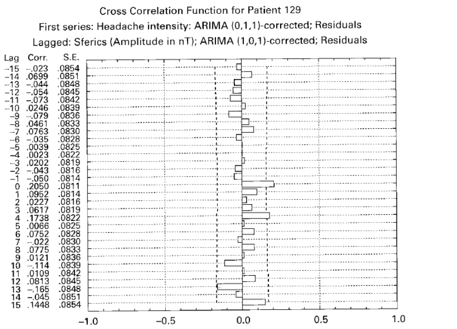
We found a significant cross-correlation in our analysis of headache and Sferics data in one of 21 patients. The idea: Sferics are ultra-short and very weak (nanoTesla) electromagnetic pulses in the atmosphere. They are mostly generated by weather fronts. At that time, we had the opportunity to use Sferics data from Prof. Betz at the TU-Munich. Headaches, some say, could also have been an evolutionary early warning signal for approaching weather hazards, so that sensitive people who got to safety in time had a survival advantage. Such correlations are also found, but only in about 5% of the headache patients we have studied.

Figure 2 reproduces the original figure from our 2001 publication [13]. The time series of headache intensity, daily data of about one year, were modelled with an ARIMA model that had no autoregressive component, an integrated component and a moving-average component (hence: 0,1,1 model). The amplitude of the sferics time series, averaged over days, was also statistically modelled with a (1,0,1) model, i.e. with an autoregressive, no integrated and a moving average component. Then the Sferics time series was shifted (“lagged”). We can see that there is a significant cross-correlation at the same point in time (lag 0) of r = .2. Not high, but significant. Since the sferics data are theoretically potential causes and the data were averaged daily, we interpreted this as a causal relationship. We found correlations in 5 other cases, but they were implausible because the time difference was negative and too large.

This shows: often such statistical models are not sufficiently good at elucidating the data structure and artificial, over-inflated and implausible contextual captures occur.

Since then, I have been extremely cautious about estimating causal relationships in time series and extremely sceptical when others report them.

This should suffice as an example to illustrate the principle of a causal time series analysis.

This perhaps also makes plausible why solely visual diagnostics are not wise for time series. After all, time series contain inherent dynamics that one must first know and understand before one can make reliable statements about their course. At best, one can make negative statements: if one would theoretically have expected clear developments, then one can see from time series, even without analysis, whether this development has occurred or not. But it is difficult to make positive statements the other way round.

I use such an example to conclude. Figure 3 reproduces data I took from the website of the Center for Disease Control in the USA on June 22, 2022. It shows the so-called “all cause mortality”, i.e. mortality from all causes, from old age to suicide, from Covid-19 to “sudden death syndrome”, from the beginning of 2018 to June 2022. The data are unadjusted and as provided by the CDC. I have only included the marker arrows to mark specific points in time, approximately.

You can see a slight excess mortality peak at the beginning of 2018. This probably stems from the fading 2017/18 flu season, which was relatively strong everywhere. This seasonal winter mortality wave can also be seen in the winter of 2018/19, but less pronounced and without a clear excess mortality, i.e. mortality that would be above statistical expectation.

This statistical expectation is marked by the orange curve (mean) and the red curve (upper confidence limit; based on the plot, these curves are close together). The winter peak in winter 2018/2019 is followed by a negative excess-mortality trough: in summer 2019, fewer people die than usual because the susceptible have already died before. Then in early 2020, Corona wave 1 begins, followed by the 2nd wave, uncharacteristically in summer. When the third wave begins in autumn 2021, the vaccination campaign also takes off, in the last two weeks of 2021. Whether the massive increase in excess mortality that then follows is related to the fact that the Corona wave was so massive, or whether vaccination into a rising epidemic wave (despite all textbook knowledge) made that wave worse, or whether vaccination was even causal for the rising mortality data, is impossible to say. But what can be seen is: neither does the otherwise usual under-mortality occur, which usually becomes visible after epidemic waves, nor does the situation relax. On the contrary: the two excess mortality peaks in September 2021 and winter 2022 are together more massive than the big one before that.

The one thing that can be said with a fair degree of certainty: Covid-19 vaccination has not led to a reduction in mortality in general, and if it has, it is not visible in these data.

Anything else would have to be tested with careful modelling of statistical dependencies and with hypothetical intervention models. We intend to present such models soon.

I hope it has become clear:

Time series analyses are complex and depend on a variety of decisions about which parameters to choose and how to model the time series. A lot of time and effort is involved. You need a lot of experience. All this makes a time series analysis susceptible to implicit biases, e.g. due to prior opinions or expectations. This became clear in the Covid-19 crisis. For here, many models were published that subsequently turned out to be wrong. Obviously, overzealous researchers wanted to provide support for certain narratives or were taken in by their own preconceptions. Researchers are, after all, only human.

Sources and literature

1. Hume D. A Treatise of Human Nature. London: Dent; 1977 1977/ / /1911.
2. Goddu A. William of Ockham’s arguments for action at a distance. Franciscan Studies. 1984;44:227-44.
3. Ockham Wv. Expositio in libris Physicorum Aristotelis. In: Etzkorn GI, editor. Opera Philosophica. 5. St. Bonventure: Franciscan Institute; 1957. p. 616-39.
4. Daunizeau J, Moran RJ, Mattout J, Friston K. On the reliability of model-based predictions in the context of the current COVID epidemic event: impact of outbreak peak phase and data paucity. medRxiv. 2020:2020.04.24.20078485. doi: https://doi.org/10.1101/2020.04.24.20078485.
5. Ferguson N, Laydon D, Nedjati Gilani G, Imai N, Ainslie K, Baguelin M, et al. Impact of non-pharmaceutical interventions (NPIs) to reduce COVID19 mortality and healthcare demand. London: Imperial College, 2020.
6. an der Heiden M, Buchholz U. Modellierung von Beispielszenarien der SARS-CoV-2-Epidemie 2020 in Deutschland. Berlin: Robert Koch Institut, 2020.
7. Chin V, Ioannidis JPA, Tanner MA, Cripps S. Effect Estimates of COVID-19 Non-Pharmaceutical Interventions are Non-Robust and Highly Model-Dependent. Journal of Clinical Epidemiology. 2021. doi: https://doi.org/10.1016/j.jclinepi.2021.03.014.
8. Flaxman S, Mishra S, Gandy A, Unwin HJT, Mellan TA, Coupland H, et al. Estimating the effects of non-pharmaceutical interventions on COVID-19 in Europe. Nature. 2020. doi: https://doi.org/10.1038/s41586-020-2405-7.
9. Dehning J, Zierenberg J, Spitzner FP, Wibral M, Neto JP, Wilczek M, et al. Inferring change points in the spread of COVID-19 reveals the effectiveness of interventions. Science. 2020;369(6500):eabb9789. doi: https://doi.org/10.1126/science.abb9789.
10. Kuhbandner C, Homburg S, Walach H, Hockertz S. Was Germany’s Lockdown in Spring 2020 Necessary? How bad data quality can turn a simulation into a dissimulation that shapes the future. Futures. 2022;135:102879. doi: https://doi.org/10.1016/j.futures.2021.102879.
11. Walach H, Lowes T, Mussbach D, Schamell U, Springer W, Stritzl G, et al. The long-term effects of homeopathic treatment of chronic headaches: One year follow-up. Cephalalgia. 2000;20:835-7.
12. Walach H, Lowes T, Mussbach D, Schamell U, Springer W, Stritzl G, et al. The long-term effects of homeopathic treatment of chronic headaches: one year follow-up and single case time series. British Homeopathic Journal. 2001;90:63-72.
13. Walach H, Betz H-D, Schweickhardt A. Sferics and headache: a prospective study. Cephalalgia. 2001;21:685-90.