Some Basic Considerations on the Methodology of Meta-analysis and Its Limitations and Possibilities
We all know those snapshots of people in motion. The more dynamic the motion, the weirder the shots – footballers with their faces contorted in rage, horses jumping with their eyes widened in fear, women who have just seen something bad and express horror on their faces, our loved ones just popping some favourite morsel into their mouths with their eyes closed and looking like they can’t count to three. And we all know that such snapshots say little about the dynamics that led to and from the image, and only in exceptional cases do they say anything about the essence of the person depicted.
Similarly, meta-analyses are snapshots in a dynamic process. In the ideal of theory, they summarize different studies and distil out a “true” effect size that is hidden in the noise of individual studies, in their lack of statistical power, or in random fluctuations. But this ideal always assumes that there really is such a thing as an “objectively true size”. We take a rain check on the examination of whether this assumption is reasonable. In practice, however, it is more like this: there are series of studies, some positive, some negative, some undecided, and depending on which one you have at hand at the moment, or which one you prefer, you decide on this or that result.
That’s where meta-analyses help to condense the results that are available at that very moment. But what if a new study comes along? After all, it could be that a new study brings to light different, new or completely contradictory results. This is not uncommon in research. Suddenly, a new approach emerges and the results of a meta-analysis crumble. Meta-analyses of anti-diabetic trials, for example, show that they have a considerable effect in keeping blood sugar in check. But foolishly, they increase mortality, something they should have prevented in the first place. That’s just one example.
[raw]
The meta-analysis essentially answers two questions:
1. is there really a statistically significant effect across the studies examined?
2. how large is the effect across all studies?
As is often the case in research, it leaves the interpretation to the researcher or the readers of the analysis.
[/raw]
[raw]
[/raw]
A new meta-analysis has just been published that tries to answer the question: do individualized homeopathic medicines work better than placebo [1]. It collected all studies that used homeopathic medicines in some form of individualized way, 32 in total, excluded those that could not be analysed and came to a positive conclusion: individualized homeopathy, it found, can be distinguished from placebo.
The so-called odds ratio was 1.53 for all studies and 1.98 for the three studies with the most reliable data. An “odds ratio” is an effect size measure that relates binary, or dichotomous, data. It is the ratio of those who improved to those who worsened or did not improve in one group relative to the number of those who improved relative to those who worsened in the other group. If these ratios are the same in each group, the odds ratio is 1.0.
This makes sense: if 20% are improved in one group and the other group is also improved, then the ratio of 20/20 is equal to 1. So arithmetically, that would be 20/100 : 20/100. That is how the odds ratio is defined. Now, it is easy to see from this that this measure is convenient in that it is independent of how large the respective numbers in the groups were; for 2/10 : 20/100 would equal 1.0 just as much as 2/10 : 200/1000.
What is also handy is that these numbers are independent of how accurately the results were determined. For example, it could be a ratio of 20 sick to 100 improved, or 20 dead to 100 alive, or 20 people whose intelligence quotient is greater than 130 to 100 whose intelligence quotient is less than that, or any other criteria determined in any way.
That’s another nice thing about meta-analyses: they translate individual study results into independent, abstract metrics. The above figures of an odds ratio of 1.53 resp. 1.98 can be interpreted as follows: a person in the treatment group – in this case “individualized homeopathy” – has a 53% higher chance of being considered improved with the criteria presented than in the placebo group, resp. a 98% higher chance. One can also use a meta-analysis to determine the statistical significance of the common number found.
This works in the same way as other significance tests: you calculate the so-called standard error and use it to determine the range within which 95% of all values lie (see my blog on statistics). If this so-called confidence range excludes the value 1.0, i.e. the value at which there is no effect, then the mean parameter found, in this case the odds ratio of 1.53, is “significant”, i.e. lies with 95% probability within a range that excludes the zero effect. That is indeed the case here.
In this respect, the researchers are justified in saying, individualized homeopathy is obviously different from placebo. And that this is the case in the studies that investigated individualized homeopathy. And only in the ones that were summarized in that meta-analysis. As soon as one, two or more studies are available that have a drastically different value, this summary can shift again. Let’s remember the photographs of moving people or animals.
So the scope of the analysis depends very much on the studies included. The authors have done a very clean job in that – this is a prerequisite – they have defined beforehand exactly which studies they want to include and exclude. After all, if they did that afterwards, they would be able to concoct the results.
What this means exactly, I will briefly demonstrate with two examples. In my view, my own study on classical homeopathic therapy of chronic headaches is still – I say this quite immodestly – one of the most methodologically elaborate clinical studies that have investigated classical homeopathy [2]. Unfortunately, it is also one of the studies with the largest negative effect sizes (about d = -0.5; I will say more about this measure in a moment). This means that its effect points in the “wrong” direction, because in this study the placebo group actually tended to be better. Now, this study was not included in the meta-analysis presented here. Why not? I asked myself and the authors. Quite simply, was the answer: we did not report means and standard deviations, but robust values such as median and percentiles, and we also did not report statistics (because the values went in a wrong direction from the hypothesis point of view and therefore no test was meaningful and necessary). Therefore, the authors were also justified in excluding them, correctly and according to meta-analytical logic lege artis. But what would have happened if these – or even more – negative studies had been included in the calculation? Possibly the effect would suddenly have disappeared. It can happen that quickly. After all, meta-analyses are a mere snapshot in the stream of knowledge.
Another example is the preceding meta-analysis by Shang et al [3]. Unlike the analysis by Mathie and colleagues that we discuss here, Shang et al did not apply any content or formal criteria. Rather, for reasons they never made clear, these authors decided to use only a subset of the studies, namely a total of 8 of the more than 120 studies that were in their collection, for the meta-analysis. Officially, they gave as a reason: those were the largest studies.
Well, one can argue for that. But then why did they add my study [2] of all things. If you take any formal criteria for “size”, then you could say: anything larger than 100 or 200 patients. Too bad, then they would have had to leave mine out; it only had 98 patients. I have never been able to shake off the impression that this selection was an arbitrary one: because with my study, the analysis remained below the significance threshold. If one orders all studies by size and adds more studies, then the analysis suddenly becomes significant. At the time, Lüdtke and Rutten [4] were able to show this very clearly in a careful re-analysis.
That means: Whether one uses meta-analysis to conclude whether homeopathy can be distinguished from placebo depends essentially on which studies one includes in the selection and which one leaves out. I do not mean to imply that Mathie and colleagues have manipulated anything. They strictly adhered to their protocol, as Robert Mathie assured me explicitly in a correspondence. Since I know him well, I have no doubt about the accuracy of this statement. From my point of view, the authors have been lucky. Let it be a few more or other studies, the situation could easily change.
You can see this in the fact that the predecessor meta-analyses come to completely contrary views, although they have essentially the same data basis at their disposal: apart from Shang [3], there would be Cucherat and colleagues [5] and Linde and others [6]. Where does this come from? Linde and colleagues decided to use as much data as possible. That is actually the normal standard. And in doing so, they found a robust, statistically significant effect.
Cucherat and others did use all the data too and got a significant result. But then they only used the studies they considered “the best” and the significance melted away. But what constitutes “the best” studies is always a matter of opinion. (See box “Study quality and meta-analysis” below) That is why Mathie and Co. applied a strict protocol in this new analysis and defined beforehand how they wanted to proceed. And, importantly, they have precisely described the intervention to be investigated: namely, classical individualized homeopathy. So only those therapy studies were included that examined homeopathy applied according to Hahnemann. This is logical.
Because if you don’t take into account the so-called “model validity”, i.e. whether what really happens or ideally should happen in a study is actually represented, then logically you are investigating a chimera. Many homeopathy studies have operationalized this suboptimally, i.e. they have answered and implemented the question “What exactly do we mean by homeopathy?” poorly. This new meta-analysis has now avoided that by looking only at “classical homeopathic individualized therapy”.
The picture that presents itself is, as I said, positive. Whether it will remain so will essentially depend on whether further studies are added that confirm this picture. Personally, I am rather sceptical for theoretical reasons, but I like to be surprised. This is also the reason why the Cochrane Collaboration regularly updates its reviews and meta-analyses. Because when a new study comes along, the situation changes, sometimes drastically. This was shown, for example, with the analysis on Tamiflu and the neuraominidase inhibitors and may be repeated here with homeopathy.
[raw]
This idea cannot be completely dismissed and stands, for example, behind the considerations on limiting the data basis by Cucherat [5]. On the other hand, there is the opinion that the amount of synthesized studies also averages out the noise that comes from the fluctuations of methodologically poor studies, which therefore should be included as much as possible. This is what the authors of the historically most influential meta-analysis on the effectiveness of psychotherapy (which at the time had triggered Eysenck’s invective), Smith & Glass, did [14]. Especially when one is at the beginning of a research development, such an approach makes sense. One can then check in a so-called “sensitivity analysis” what happens if one includes and excludes studies with a certain design or other characteristics and repeat the analysis. Such a more exploratory approach then very often gives valuable clues as to which factors influence the effect size, the so-called moderating variables.
Some authors choose to include only the most methodologically stringent studies in a meta-analysis and exclude all studies that, for example, are not randomized or were not conducted against an active or placebo control. This was also done in the analysis presented here by Mathie and colleagues. Elaborate meta-analyses code the study quality with a very complex coding scheme, which of course has to be defined beforehand. If one wishes, one can then express the study quality in a numerical value, which one uses to weight the studies. Then only the studies that are really very good would be included in the analysis at 100% and the others with correspondingly less weight. Wittmann and Matt did this at the end of the 1980s and were thus able to show that careful studies document strong effect sizes of psychotherapy, whereas methodologically sloppy studies tend to leave psychotherapy worse off [15].
The Cochrane Handbook and various recent analyses choose a middle course: they propose to assess the individual studies according to their “risk of bias”, i.e. according to how great the risk is of being mistaken due to expectations and such. In principle, this is a rough assessment of the internal validity of a study. The most important criteria are documented: whether a study was randomized or not, whether the allocation to the groups was blinded, whether the participants and the investigators were blinded, whether there was a high drop-out rate (this provides information about the quality of the organization of a study and the acceptance of the intervention). Sometimes it is also documented whether target criteria were set a priori. One can then use these assessments descriptively, or one can use them to calculate sub-analyses with subgroups of studies, which provide information about whether methodologically less stringent studies tend to overestimate the effect and thus whether methodological quality plays a role or not. Sometimes it does, sometimes it does not. One must also look closely: the authors do not always get these ratings right. Often assistants are used who know too little; or a study may not report carefully enough, for example because it was only published as a “research letter” with little space. In such a case, it would be necessary to obtain the information from the authors.
To process methodological study quality as a variable quantitatively, i.e. in the sense of weighting, is very time-consuming. That is probably why very few authors do it. Many study details cannot be obtained from published reports, but would have to be requested from the authors. This is usually only possible with recently published studies.
This reasoning and these arguments are also used by some authors to reduce complexity and to apply relatively strict inclusion and exclusion criteria. That makes life easier for them because less material has to be processed. Whether they are doing right by the matter by doing so is quite another question. Personally, I don’t think it makes sense to restrict meta-analyses only to randomized studies. This is because it takes away the possibility of exploratory investigation of which variables contribute to the variation of the effect (see below: Homogeneity and moderator analysis box).
[/raw]
One other point I wanted to make: Mathie and colleagues used the odds ratio as a metric. This is, as I said, an effect size related to dichotomous measures and variables. Such variables occur in nature, but are more likely to be generated by us through reduction of information. They occur naturally when we consider properties such as “dead” and “alive”. These are clearly dichotomous. But most other properties and variables are actually naturally continuous: health and disease, for example, tend to be on a continuous spectrum, as do well-being, energy, quality of life, severity of symptoms, perceived inner satisfaction, blood pressure readings, immunological parameters, intelligence, and so on. It is only our tendency to reduce information that then makes it something like: “healthy” vs. “sick”, “has a diagnosis” or “does not have a diagnosis”, “has a relapse” or “does not have a relapse”, “is clever” or “is stupid”, “is happy” and “not depressed” or “unhappy” and “depressed”.
We see: As a rule, the use of a dichotomous measure, and thus of the odds ratio as a ratio, is due to information reduction and occurs naturally only where mortality or the occurrence of a series of events – hospitalization, surgery or rehab needed – is dichotomously scored. Doctors like to do this because they think it increases clinical relevance. After all, in medical practice, decisions have to be made that are also dichotomous: Do we operate or not? Do we give medication or intervention or not? Does the person need to be monitored clinically, or is he allowed to go home? And so some studies summarized in this meta-analysis are implicitly built on such dichotomous outcome measures.
In very many cases, however, we use continuous measures. This is again a matter of academic culture. Psychologists, for example, try to construct measures that are as continuous as possible, for example by combining many individual questions, so-called “items”, to produce a continuous value on a scale. This is done in classical tests such as intelligence tests or personality questionnaires. But also with so-called clinical outcome measures, which are supposed to measure clinical changes, such as depression questionnaires, quality of life questionnaires, pain scales, symptom scores, wherever possible we try to map the continuity of what is happening to us humans in continuous measures.
Then studies report, for example, different values in a measure of quality of life between two groups, or different mean pain scores, or number of days a symptom occurred, and so on. In such cases, we are dealing with continuous measures. These are usually reported as mean values found in a group, summarizing the values in that group, and the dispersion of these values in a group. Sometimes robust measures are taken, such as the median, which describes the point above which 50% of all measured values lie. If the distribution is regular, the mean and median are usually very close. Only when there are large outliers does the mean overestimate or underestimate, and then one prefers to take the median.
Such studies are summarized in a meta-analysis using the effect size measure “d” (for “difference”), which is sometimes also referred to as “SDM” (“standardized mean difference”) or in a certain form as “g” if “d” has been reduced by a factor that takes into account the different study size. I wrote about this in some detail in my blog on “Power” (“The Magic of Statistics”) and will just briefly repeat here:
“d” is obtained by subtracting the mean values of the two groups from each other, i.e. by forming a difference between the groups. This shows the size of the difference between the groups. If we were only dealing with values of the same category, e.g. only blood pressure values, or only intelligence values, or only values of a certain depression scale, then we could leave it at that, because we have quantified a difference. But because we often have very different dimensions in front of us, we have to come up with a trick to make the differences comparable. This is done, for example, with the odds ratio, by looking not only at the improved patients in each group, but at the improved patients in relation to all patients.
With continuous measures, one manages this trick of making comparisons by so-called “standardization” (hence SDM): one divides the difference by the standard deviation, i.e. the dispersion of the values in a group. The dispersion is defined by the deviation of the individual values from the mean [7]. To make the differences comparable, they are divided by the standard deviation and thus standardized. This means: one can compare the differences from, say, differences measured in millimetres of mercury column, with differences measured with an intelligence test or with differences measured with a quality-of-life scale. The difference is a dimensionless number “d” that can at best be interpreted as a multiple number of a standard deviation. So my own study’s negative effect size d= -0.5, mentioned above, was about half a standard deviation worsening for the treated group.
Personally, I find meta-analyses based on effect size d a bit more informative. But essentially it depends on what measures were used in the majority of the original and pooled studies. The approach of many meta-analysts now is to include in their analysis only those studies that use or allow the measure they favour for calculation, and ignore the others. This is bad practice. Some analyses then rather conduct two separate analyses, one for each metric. This is a pity, because it is precisely the strength of meta-analysis that is lost, namely bundling the statistical power of the individual studies and thus arriving at a more compact statement. The meta-analytical specialists usually transform the metrics into one another. There are various ways to do this. For example, one can transform odds ratios and similar measures via an arcsine transformation into a value that can be interpreted as a d-value. Or one can apply a formula presented by Hasselbald & Hedges [8], with which one can transform into one direction and into the other, i.e. convert d-values into odds ratios and vice versa. To my knowledge, this is what Linde’s analysis [6] did. The analysis presented here used a simpler method published later, but also used by the Cochrane Collaboration, which essentially provides good estimates [9]. Here, the transformation from continuous values, i.e. d to odds ratio, was made awkwardly because, after all, most studies did indeed have continuous outcome measures and information is lost as a result.
I reproduce below the original graphic of the summary analysis:
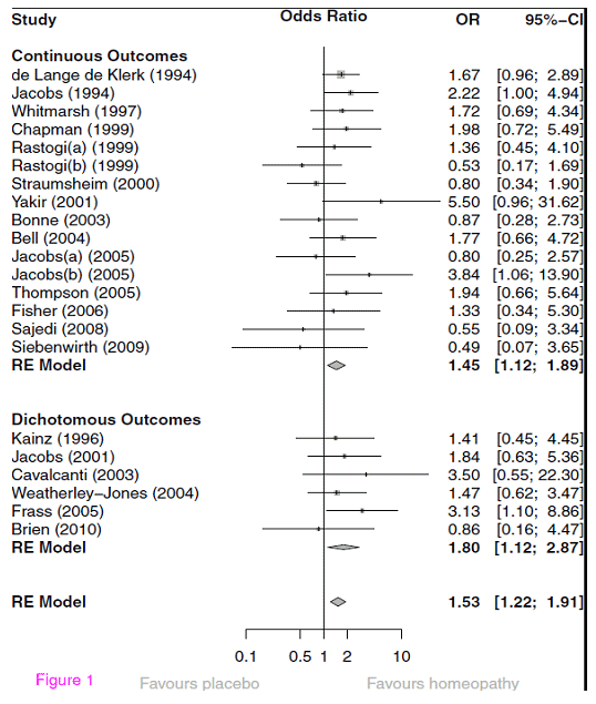
This figure is standard in meta-analyses. Let’s give a little attention to its interpretation. First, we see that most studies used continuous outcome measures; however, they were transformed into odds ratios using the transformation discussed above. Then in the lower section are the studies that do indeed report dichotomous outcomes and are also correctly mapped with odds ratios. One could have imagined a reverse procedure here. On the left, the individual studies are named, each line represents a study and the number under the heading “OR” indicates the “odds ratio”. The graph in between shows the same number and the corresponding confidence interval graphically as a dot of different size. The 95% confidence interval, listed numerically in square brackets next to the OR and graphically as a dash, shows how confident the estimate of the OR is and indicates the individual significance of the study.
[raw]
.
In other words, the variable (what is measured) and the parameter (what underlies what is measured) are then identical. In practical terms, however, one will never be able or willing to capture all values. That is the trick of statistics, to avoid total surveys if possible. This trick is paid for by the uncertainty of the estimate. It is immediately obvious that the precision of the estimate is directly related to the size of the sample (and its representativeness). For example, if we measure the blood pressure of all the people in a city, then our measurement has no uncertainty and the mean blood pressure we measured is identical to the mean blood pressure of the population in the city. If we only do this for every 10th inhabitant, then we estimate the mean blood pressure of the population on the basis of our data and of course have to reckon with an uncertainty.
Mathematically, this is expressed by standardizing again, and in this case by taking the root of the total number of our measurements. This means: the more values we have, the lower our estimation uncertainty becomes. The confidence interval makes use of this fact. Because the standard error of the estimate, it is called, can in turn be interpreted as following a standard normal distribution, where the standard error represents the standard deviation of that distribution. Because the total area of the distribution is standardized and gives “1”, the area under the curve can be interpreted as the probability. Thus, with the help of this standard error, one can calculate under which area 95% of all values will lie. This is always 1.96 * standard error (which in this case represents the standard deviation of this distribution) of all values to the left and right of the mean of this distribution, because the area to the left of the ordinate points of + or – 1.96 together make up 5% of the area of the curve.
Therefore, one can interpret such confidence intervals in such a way that 95% of all estimated values will lie within these value limits, or, in other words, that one only makes an error in 5% if one says that the real value lies within this value range.
[/raw]
So, in the meta-analysis example, the listed confidence range of the effect size estimate is the range in which there is a 95% probability of finding the true value. Because the size of the underlying study is included in the calculation of the standard error, these confidence intervals vary accordingly. Small studies, such as Yakir’s pilot study or Siebenwirth’s study, have very large confidence intervals, while relatively large studies, such as Elli de Lange de Klerk’s, have small confidence intervals.
In the graph, the line is solid at the OR of 1. This is the zero-effect line. It marks the value where there is no effect at all, namely at an OR of 1. Everything to the left of it denotes a negative effect, where a study shows placebo to be better. Everything to the right of it demonstrates an effect. If the line of the confidence interval crosses the zero effect line, the effect of the individual study is not particularly clear or statistically significant. One can immediately understand that this depends on two variables: how large the effect of the study is, and how extended the confidence intervals are or how large the study is. This is another way of saying what I have already said in my blog about statistical power (“The Magic of Statistics”): Whether a study becomes significant depends on the effect size and the study size. We can see from the graph: few studies are independently significant because they have large effect sizes.
Now, below the individual studies, we see a so-called “diamond”. This is the estimator for the total, averaged effect size of all the studies shown above, and its confidence range, also shown in brackets next to it. If this does not cut the line, i.e. the confidence range does not contain the value “1.0” or smaller, then it is statistically significant. We see two such summary estimators: above one for the studies with continuous outcome with a significant odds ratio of 1.45, below one for the studies with dichotomous outcome with an odds ratio of 1.80 (with a larger confidence interval, but also not cutting the line and therefore significant). And finally, an overall estimate for all studies. This is also in the significant range, with an odds ratio of 1.53 and a confidence interval that does not include 1.
To the left we read “RE Model”. This means: A statistical model was applied here that assumes a random effects model (RE model). This means the following: One could come up with the idea that all studies that investigate a certain question converge on a “true” value in the end. This would mean statistically: each study can be expressed as a measured value plus a deviation from this true value, a so-called “error”. This assumption is usually problematic because we do not know whether it is really true. Therefore, a more conservative, and in many cases more plausible, assumption is that a meta-analysis estimates values based on a true value, together with an error, but all still varying by an unknown, random variation around this true value. Why, we do not know, but we suspect that there is such variation. This is the “random effects” model. It manifests itself in the fact that the estimate of the values is less precise and is therefore statistically more conservative. Practically, one always adopts such a model when dealing with a very heterogeneous group of studies, as is the case here. So by using a “random effect” model like this, the estimate becomes conservative and is therefore more credible.
So far, all is well: we have a precise estimate of mean effect sizes of individualized homeopathy versus placebo, showing that homeopathically treated patients have about 53% better chances of recovery than placebo-treated patients, which is statistically significant. That’s not bad, I think. But what exactly does it mean? What does it say?
For better orientation, we transform this OR [10] and get an approximated d = 0.235 or d = 0.23. This is a rather small effect. To be able to classify it, we put it in relation. Stefan Schmidt has just published a basic introduction to the experimental effects of parapsychology [11]. There is a summary of effect sizes (all significant) of recent meta-analyses within parapsychology, which I reproduce in excerpts:
| Paradigm [12] | Effect size d | p-value |
| Presentiment (Mossbridge 2012) | 0.21 | 2*10-12 |
| DMILS (Schmidt 2004) | 0. 11 | 0.001 |
| Remote Staring (Schmidt 2004) | 0.13 | 0.01 |
| Attention Facilitation (Schmidt 2012) | 0.11 | 0.030 |
We see the effect size that homeopathy shows over placebo is slightly larger than the largest of the parapsychological effects. What about clinical medicine? Here a recently published review helps us, that compared the effect sizes of psychiatric-pharmacological interventions with those of all possible standard medical procedures [13]. I reproduce the effect sizes described there in excerpts:
| Disease pattern | Effect size d |
| Blood pressure reduction: | 0. 54 |
| Cardiovascular events: | 0.16 |
| Prevention of cardiovascular disease and stroke: | 0.06 to 0.12 |
| chron. Heart failure: | 0.11 |
| Rheumatoid arthritis (methotrexate): | 0.86 |
| Acute migraine: | 0.41 |
| preventive: | 0. 49 |
| Asthma: | 0.56 |
| COPD (chronic obstructive pulmonary disease): | 0.36.; 0.20 |
| Diabetes/metformin: | 0. 87 |
| Hepatitis C: | 2.27 |
| Oesophagitis: (proton pump inhibitors) | 1.39 |
| Ulcerative colitis: | 0. 44 |
| MS exacerbation: | 0.34 |
| Breast cancer (polychemotherapy): | 0.24 |
| Antibiotics for otitis: | 0. 22 |
| for cystitis: | 0.85 |
| For psychiatric disorders: | |
| Schizophrenia: | 0. 30-0.43 (responder) 0.51-0.52 (rating) |
| Depression: | 0.32 (rating) 0.24-0.30 (responder) |
| Relapse prevention: | 0.53-0. 92 (with lithium) |
| Compulsive disorder: | 0.44 (symptoms) 0.53 (response) |
| Bipolar disorder: | 0.40-0.53 (symptoms) 0.41-0. 66 (Response) |
| Relapse Prevention: | 0.37-1.12 |
| Panic: | 0.41 |
| Dementia: | 0.26-0.41 |
| ADHD: | 0.78 |
We see two things from this comparison table: first, even in conventional medicine, effect sizes vary enormously between a small effect size of d = 0.11 in preventing heart failure or d = 0.06 in preventing stroke and very large ones like d = 2.27 in hepatitis C (though only a few studies). The median effect size is d = 0.4. The aim of the study [13] was to find out whether psychiatric interventions are comparable to conventional medical interventions. They are and, however, have a somewhat smaller range of variation. But there are also relatively marginally effective interventions in psychiatry, such as the treatment of depression when a hard criterion (does a patient have a positive response to therapy?) is asked, or in the therapy of dementia. Here, too, the mean effect size of d = 0.4 is about equal to that of conventional treatments.
Homeopathy, then, with its d = 0.23, does not look so bad. We must bear the following in mind when interpreting this: The meta-analysis by Mathie and colleagues was deliberately designed to estimate effect sizes conservatively. Many studies were not included in the analysis because they did not meet the criteria, precisely so as not to dilute or inflate the effect. And the comparison takes place, as an expert once wrote to me, “between a placebo and another placebo”, because pharmacologically the homeopathic medicines contain “nothing”, at least nothing that can be determined and weighed. And in this respect, this result is sensational from a scientific point of view. For it should not have occurred at all.
Will it end the debate about homeopathy? Do we now know for sure that homeopathy is not a placebo? No, I don’t think so. For one thing, a meta-analysis is one snapshot of a dynamic event. For another, the result depends on so many presuppositions, on the inclusion and exclusion of studies, for example, that another working group, using the same study material but with slightly different criteria or procedures, could come to different results, as has often happened in other fields. Because, as most people overlook, meta-analyses are, in my view, research tools that help us find new ways and clarify whether we already know enough in a pragmatic sense and how this knowledge, cumulatively, is to be quantified. How this knowledge is then to be classified and evaluated is a completely different question. The answer depends on how large an effect has to be for us to be interested in it, what other options there are for therapy, how costly they are, how fraught with side effects, etc.
Meta-analysis was originally an invention of psychologists to settle the dispute over whether psychotherapy works or not [14, 15]. It stimulated constructive dialogue, at least at that time. The original question has become even more complex rather than answered. One could say: something about psychotherapy seems to work. But what exactly? With whom exactly? With which method? And why? Such questions are usually investigated meta-analytically through moderator analyses and then in further process research studies (see box moderator analysis).
[raw]
In Mathie and colleagues’ analysis, there was no heterogeneity. In our own meta-analysis on mindfulness in children [16], there was a lot of heterogeneity. We were able to resolve it by noting that the studies with the largest effect sizes all came from a research group that had studied particularly intensive training in rather older adolescents. In this way, meta-analyses also help to clarify the significance of individual variables for the effect under investigation, provided that the variable has been recorded beforehand and there are enough studies in the portfolio to calculate such analyses. The analysis by Lüdtke and Rutten [4] can also be seen as a catch-up moderator analysis to the meta-analysis by Shang [3], which shows that Shang’s result is not robust enough to pass as a scientific fact. This is because the aim of moderator analyses is to document the robustness of the analysis against violation of assumptions or under different scenarios.
[/raw]
All these additional questions are still hotly debated today, 35 years after Smith and Glass’s original analysis. So can Mathie’s analysis settle whether homeopathy is placebo? No, it can’t. But it does present some good arguments that show that the question is not simply off the table. Because if it were, then we wouldn’t necessarily have expected a significant effect size here. But why should that be? How can we explain it? And: should we care? The analysis cannot answer all these questions.
In my opinion, they should be of interest to us. If the analysis had been about a normal, conventional medical treatment method, where one thinks one knows the underlying pharmacological mechanism and which is used in every hospital, there would most likely have been a comment like: “Well, the effect is not as strong as we had hoped for. But it is clearly significant and still better than placebo.” Now, the intervention is known but controversial, and we have no idea at all how it could work. That is precisely why the procedure, homeopathy, and the result of the analysis should begin to interest us.
But this requires many other steps. Above all, a discourse on what makes a finding scientifically relevant. I think the analysis at least opens up the dialogue on this and has in any case robustly documented a finding that should be of interest to all those who do not yet believe we already know everything. After all, how can it be that something that is not there versus something that is not there produces a clear, statistically significant and also clinically not irrelevant effect? What the meta-analysis tells us is that this effect occurs by chance in less than one in 1000 cases. This does not rule out chance, but it does not make it particularly attractive as an explanation. What can explain such an effect to us?
So meta-analysis opens up questions rather than answering any. And asking questions has always been the silver bullet of science: To not think you already have answers to all the questions. Which we should leave to dogmatics and religion. In this respect, meta-analysis is a scientific method. It usually produces more questions than it answers, even if it answers some questions that were asked before. Now we know: statistically speaking, individualized homeopathic therapy is rather not placebo therapy – at least with the data we have at the moment. But that actually leaves us perplexed. Because now we might have to think about how that could be. Or do new studies. Or both. It just never stops…
That’s why those interested in definitively settling questions should become priests, not scientists.
Sources and references
- Mathie, R. T., Lloyd, S. M., Legg, L. A., Clausen, J., Moss, S., Davidson, J. R., et al. (2014). Randomised placebo-controlled trials of individualised homoeopathic treatment: sytematic review and meta-analysis. Systematic Reviews, 3(142). doi:10.1186/2046-4053-3-142 [online verfügbar]
- Walach, H., Gaus, W., Haeusler, W., Lowes, T., Mussbach, D., Schamell, U., et al. (1997). Classical homoeopathic treatment of chronic headaches. A double-blind, randomized, placebo-controlled study. Cephalalgia, 17, 119-126.
- Shang, A., Huwiler-Münteler, K., Nartey, L., Jüni, P., Dörig, S., Sterne, J. A. C., et al. (2005). Are the clinical effects of homeopathy placebo effects? Comparative study of placebo-controlled trials of homoeopathy and allopathy. Lancet, 366, 726-732.
- Lüdtke, R., & Rutten, A. L. B. (2008). The conclusions on the effectiveness of homeopathy highly depend on the set of analyzed trials. Journal of Clinical Epidemiology, 61, 1197-1204.
- Cucherat, M., Haugh, M. C., Gooch, M., Boissel, J. P., & HMRAG Group. (2000). Evidence of clinical efficacy of homeopathy. A meta-analysis of clinical trials. European Journal of Clinical Pharmacology, 56, 27-33.
- Linde, K., Clausius, N., Ramirez, G., Melchart, D., Eitel, F., Hedges, L. V., et al. (1997). Are the clinical effects of homoeopathy placebo effects? A meta-analysis of placebo controlled trials. Lancet, 350, 834-843.
- Mathematically precise, the scatter is determined as follows: First, the differences of the individual values from the mean value are formed and squared; thus, all negative signs disappear. Then these so-called squares of deviation are added up and averaged, i.e. divided by the number of differences or values that have been included in the calculation. This means: here, too, a standardization takes place on the number of values; in this way, scattering of values in large and small samples becomes comparable. In order to get back to the original metric – we squared before – the root of this value is taken. The value found in this way is called the “standard deviation”. The initial value, i.e. the sum of the standardized and squared deviations from the mean, is called “variance”.
- Hasselblad, V., & Hedges, L. (1995). Meta-analysis of screening and diagnostic tests. Psychological Bulletin, 117, 167-178.
- Chinn, S. (2000). A simple method for converting an odds ratio to effect size for use in meta-analysis. Statistics in Medicine, 19, 3127-3131. An odds ratio is first logarithmised. Then it can be converted to an effect size d by dividing the log odds ratio by 1.81, as well as the standard deviations. This approximates the effect size d because the logistic distribution is quite similar to the standard normal distribution and, as a projection, is linear everywhere except at the outer edges, with a variance of pi2/3-2, which is 1.81. This gives the confidence intervals of the standard normal distribution. Thus, the confidence intervals are smaller because the statistical power increases.
- (About the procedure as described in [9]: we take the natural logarithm of 1.53; result: 0.425. We divide this by 1.81: d = 0.235
- Schmidt, S. (2014). Experimentelle Parapsychologie – Eine Einführung. Würzburg: Ergon, S. 99.
- Presentiment studies are those in which a physiological measure is used to investigate whether people anticipate scary images before they are shown. DMILS studies are those in which someone influences another person’s autonomic arousal over distance. Remote Staring are studies where one person looks at another’s image on a screen, and autonomic arousal is measured in the person being looked at. And Attention Facilitation is about a group of people across distance randomly helping another person to focus on a stimulus.
- Leucht, S., Hierl, S., Kissling, W., Dold, M., & Davis, J. M. (2012). Putting the efficacy of psychiatric and general medicine medicatin into perspective: review of meta-analyses. British Journal of Psychiatry, 200, 97-106.
- Smith, M. L., Glass, G. V., & Miller, T. I. (1980). The Benefits of Psychotherapy. Baltimore: Johns Hopkins University Press.
- Matt, G. E. (1989). Decision rules for selecting effect sizes in meta-analysis: a review and reanalysis of psychotherapy outcome studies. Psychological Bulletin, 105, 106-115.
Matt, G. E. (1997). What meta-analyses have and have not taught us about psychotherapy effects: A review and future directions. Clinical Psychology Review, 17, 1-32.
Wittmann, W. W., & Matt, G. E. (1986). Meta-Analyse als Integration von Froschungsergebnissen am Beispiel deutschsprachiger Arbeiten zur Effektivität von Psychotherapie. Psychologische Rundschau, 37, 20-40. - Zenner, C., Herrnleben-Kurz, S., & Walach, H. (2014). Mindfulness-based interventions in schools – a systematic review and meta-analysis. Frontiers in Psychology; 5: Art. 603. doi:10.3389/fpsyg.2014.00603 [available online]